
Modeling of the wave propagation in the solid bar
Sergiyenko A. M., Qasim M. R.
Computer Engineering Department of NTUU “Igor Sikorsky Kyiv Polytechnic Institute”, Kyiv, Ukraine
Introduction. The acoustic processes in solids are usually modeled in the computers using the finite difference method, which affords the huge computational resources. On the contrary, the digital waveguide (DWG) method provides the high-speed computations utilizing much less computation volume [1]. A lot of successful examples of the DWG implementation are shown in modeling and sound synthesis of the string and wind musical instruments [2,3]. But this model does not take into account the dispersion in the sound propagation.
In this work, a DWG method modification is proposed which provides the modeling of the sound dispersion in the solid bar.
DWG model basics. DWG is a digital model of the wave propagation in the ideal waveguide. It is based on the principles, described in the work [4], but adapted to the sound wave modeling. The forward fi = Rvf and backward bi= −Rvb waves are considered in the i-th point of the waveguide, where fi and bi are the pressure of the forward and backward (reflected) waves, respectively, R is the wave impedance, vf, vb are the particle velocities. For the solid cylinder with the cross-section A the impedance is equal to R = ρc/A, where ρ is the matter density, c is the velocity of the longitudinal waves. The real pressure value is equal to u = fi + bi.
In the DWG model, the signals are sampled at a sampling frequency of Fs which is at least two times greater than the maximum considered frequency. Then the i-th section of the waveguide of the length L looks like two delay lines at n = L/(co Fs )cycles, where co is the wave velocity. The homogeneous parts of the waveguides are connected together by the adapters, also called as the scattering nodes. The adapter function is designed to satisfy the Kirchhoff’s law. For the case of joining two wave guides:
vb 1 = rvf1 + (1 − r)vf 2; vb 2 = (1 + r)vf 1 − rvf 2; (1)
where r = (R2 − R1)/(R2 + R1) is the reflection coefficient. Similarly, when three waveguides are connected, then the adapter node calculates the following formulas:
Ao = (2g1 − 1)A + 2g2 B + 2g3 C; (2)
Bo = 2g1 A + (2g2 − 1)B + 2g3 C;
Co = 2g1 A + 2g2 B + (2g3 − 1)C;
where A, B, C are the waves entering the node, Ao , Bo , Co are the waves leaving the node, g1, g2, g3 are the specific impedances of the waveguides, and g1 + g2 + g3 = 1, gi = Ri /(R1 + R2 + R3).
DWG model improvement. Due to the theory, the primary longitudinal wave with the phase velocity cp, and the secondary transverse wave with the velocity cs, cs < cp are propagated in the solid bars [5]. The waves of different types can be transformed into each other interacting with the media boundaries. Besides, the longitudinal waves have a dispersion, i.e. its velocity cp depends on the wave length λ. The velocity cp in a cylinder is approximated as follows [5]:
cp = co (1 − ν2 p2 a2 /λ2 ) = f (λ), (3)
where ν is the Poisson ratio, which is equal to 0.29 for the steel, a is the cylinder radius. Therefore, the DWG model has to be corrected according to this formula.
The modified DWG model of a bar is illustrated by Fig.1. This model consists of the left LA and the right RA adapters, the waveguide P of longitudinal waves, and the waveguide S of transverse waves. Each three port adapter compute the equations (2). Its port, which means the bar end, is connected to the network, which implements the wave reflection with the suppression factor sL or sR due to (1). The actuating signal vin is fed to the model through an adder.
The waveguide S performs the delay to the given number of clock cycles and some wave attenuation. The waveguide P does the same but it has a set of channels. Each of them has the separate frequency band, delay, and attenuation depending on the respective wave length λ according to (3).
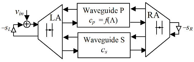
Figure 1. Structure of the solid bar model
Experimental results. Up to eight channels of the waveguide P are implemented on the basis of the allpass filters described in [6]. Each channel has the dynamically tunable band pass filter, which is implemented as is shown in [7]. The resulting amplitude-frequency characteristic of the waveguide S is shown in Fig.2. Here, the frequency f is measured in parts of the sampling frequency Fs, the characteristics of two neighboring channels are shown as well.
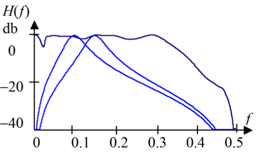
Figure 2. Amplitude-frequency characteristic of the waveguide P
The model was actuated by a narrow ultrasound impulse, and the velocity v was measured in the output of the adder node (see Fig.1). The time diagram of it which represents the wave signal is shown in Fig.3. This diagram shows that the waves are really dispersed after the propagation through the bar model.
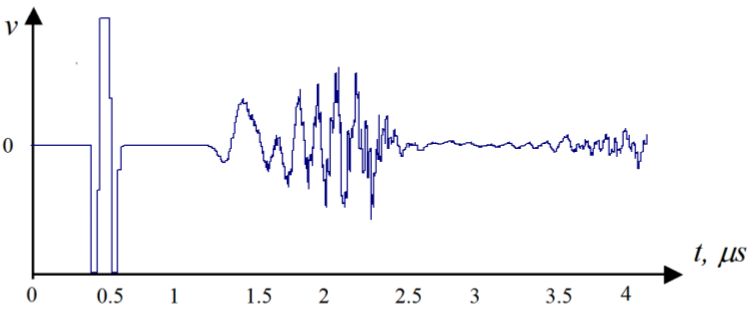
Figure 3. Time diagram of the wave signal in the solid bar model
The model is described by the VHDL language and therefore, it can be implemented both in the VHDL simulator and in FPGA. The model described in the style for the synthesis and configured in Xilinx Spartan-6 FPGA contains 2680 logic cells, 60 DSP48 blocks, 16 BlockRAMs, and provides the sampling frequency Fs < 100 MHz. This provides the modeling in real time.
Conclusion. A modified DWG method for modeling the solids is proposed which takes into account the dispersed wave propagation. The method is based on the digital wave guides which delay is depending on the wave length. An example of the solid bar model described in VHDL shows the effectiveness of this model.
References.
- D. R. Bergman “Computational Acoustics: Theory and Implementation”. J.Wiley and Sons, Ltd. 2018. 296 p.
- J. O. Smith III “Physical Modeling Using Digital Waveguides”. Computer Music Journal V.16. 1993. No4.pp.74-91.
- M. Karjalainen, and C. Erkut “Digital Waveguides versus Finite Difference Structures: Equivalence and Mixed Modeling”. EURASIP Journal on Applied Signal Processing 2004. No7. pp. 978–989.
- A. Fettweis “Wave digital filters: Theory and practice”. Proc. IEEE, V74, 1986. No2. pp. 270 – 327.
- H. Kolsky “Stress Waves in Solids”. Dover Publications Inc. 2012.
- P. A. Regalia, S. K. Mitra, and P. P. Vaidyanathan “The Digital All-Pass Filter: A Versatile Signal Processing Building Block”. Proc. IEEE. V.76. 1988. —76, No1. pp. 19—37.
- А.М Сергиенко, Т.М Лесик “Перестраиваемые цифровые фильтры на ПЛИС”. Электронное моделирование, Т.32. 2010, No6. C. 47-56.(A. M. Sergiyenko, and T. M. Lesyk “Tunable digital filters in FPGA”Electronic Modeling. V.32. 2010.No6. pp. 47-56).