Gauss noise generator VHDL-model and its use in DSP
A.Sergyienko
National Technical University of Ukraine “KPI”,
Email: aser@comsys.kpi.ua
In this article we propose to do a set of experiments with the simple signal generator models as well as with some algorithms of simple but effective processing of the derived signals.
Signal generators are widely used for the DSP unit testing. For this purpose the sine wave generator is widely used due to the fact that the sine wave is traversed the linear system without its form damage. Such a generator is proposed here
http://kanyevsky.kpi.ua/wp-content/uploads/2017/09/labexercise-1.pdf.
The noise signal has the wide spectrum. Therefore, its use helps to estimate the frequency response of the system. The noise is added to the testing signal to estimate the filtering property of the system. Consider we input the special form signal to the system. Then this system is valued as good one when the output signal follows the form of the input one.
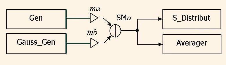
Here we consider the description of the special form generator Gen and Gauss noise generator Gauss_Gen. We do here a set of experiments using the network in the Fig.1.
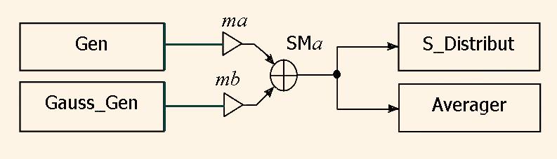
The other units in the Fig. 1 are statistical analysis unit S_Distribut, and averaging unit Averager.
The Gauss noise generator is based on the central limit theorem of the statistics. Due to the theorem, if the probable datum is the sum of a set of N independent probable data then this sum has the binomial distribution, which approaches to the Gauss, or normal distribution.
The Gauss noise generator described by VHDL looks like the following.
library IEEE;
 use IEEE.STD_LOGIC_1164.all;
 use IEEE.math_real.all;
 entity Gauss_Gen is
  generic(nn:natural:=1; --power of the binomial distribution <16
  m:REAL:=0.0	 -- mean output value
	);
   port(
	CLK : in STD_LOGIC;
	RST : in STD_LOGIC;
	DATA_OUT : out REAL:=0.0
	);
   end Gauss_Gen;
 architecture Model of Gauss_Gen is
     	type arri is array (0 to 15) of integer;
      	type arrr is array (0 to 15) of real;
 begin
 SFR:process(clk,rst)
  variable s1:arri:=(3,33,333,3,4,5,6,7,8,9,11,22,33,others=>55);
  variable s2:arri:=(5,55,555,50,6,7,8,9,5,6,7,21,33,others=>22);
  variable r:arrr:=(others=>0.0);
  variable s:real:=0.0;
      	begin
           if rst='1' then
              DATA_OUT<=0.0;
           elsif  clk='1' and clk'event then
 		s:=0.0;
       	for i in 0 to nn-1 loop    -- nn noise generators
                   UNIFORM (s1(i),s2(i),r(i));
                   s:=s+r(i);
       	end loop;
        	DATA_OUT <= 2.0*(s/real(nn)-0.5)+ m;
           end if;
      end process;
  end Model;
Unit Gauss_Gen has two parts. The first one has nn parallel uniform noise generators. The data uniformly distributed at the interval [0.0,1.0] are generated by the congruent algorithm, which is performed by the procedure UNIFORM. The second part is an adder, which adds nn generated random numbers. The sum is divided by nn and adjusted to the interval [-1.0,1.0].
The figure nn is the generic variable. By nn = 1 the generator generates the uniform noise, by nn = 2 it generates the triangle distribution noise, and by nn > 10 the output signal is practically the Gauss noise.
The signals from the generators Gen and Gauss_Gen are added in the adder SM after multiplication them to the scale factors mа, mb, respectively. As a result, we get the complex signal х(n), which we will test. The scaling adder model is the following.
      library IEEE;
      use IEEE.STD_LOGIC_1164.all;
      entity ADD2 is
      	generic(ma:real:=1.0;
      	mb:real:=1.0);
      	 port(	 A, B: in REAL;
      		 S : out REAL:=0.0 );
      end ADD2;
      architecture ADD2 of ADD2 is
      begin
      	S<=ma*A + mb*B;
      end ADD2;
When we build the histogram of the signal х(n) probability distribution then its statistical properties can be estimated. The histogram calculation is implemented as the following. The value (n) representation interval, say, а < х(n) < b, is divided to k subintervals of equal length. і-th subinterval as well as 0-th subinterval х(n) < а and k+1 –th one b < х(n), responses to the natural number Мі,. This number is equal to the number of samples х(n), which enter the respective i-th subinterval. The i-th subinterval is called as i-th bin.
Consider the subinterval length is с = (b – а)/k, and the limit of the і-th bin is di = a + i*c. Then after the analysis of the whole signal sequence x(n) in the і-th bin we derive the number of j samples х(n), so that di-1 < х(n) < di. The 0-th bin for samples х(n) < а, and k+1-th bin for samples i>b < х(n) are exclusions.
By processing the signal х(n) the array M of k+2 integers. If а < х(n) < b , then the number of bin is calcula
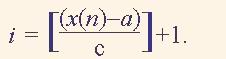 (1)
(1)
Here the brackets [] means the rounded value. Deriving the index by the formula (1) a one is added to the i-th bin, i.e. to the array element М(і). Such a calculation is repeated for all data х(n).
If the length of the sequence х(n) is equal to N then the probability distribution function is calculated by the formula
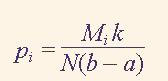 (2)
(2)
The selection of parameters а, b, k, in general, depends on hypothesis of the signal х(n) distribution, method of data sampling and N . Surely, the number of bins must be less than о√N , or than the number quantization levels of х(n). The parameters а, b, k are corrected after some estimating cycles of histogram deriving.
The probability density histogram is derived in the unit S_Distribut:
   library IEEE;
   use IEEE.STD_LOGIC_1164.all;
   entity S_Distribut is
   generic(channels:natural:=100;
      		drange:real:=2.0;
     		dmin:real:=-1.0);
      	port(	CLK, RST: in STD_LOGIC;
      		DATA : in REAL:=0.0;
      		ADDR : out INTEGER;
      		DISTRIB : out INTEGER);
   end S_Distribut;
   architecture MODEL of S_Distribut is
      	type Tarr is array (0 to channels+1) of natural;
      	signal Distr_arr:Tarr:=(others=>0);
      	signal addri,aa:natural;
      	signal even: STD_LOGIC;
   begin
     process(CLK)
        variable addrw:integer;
     begin
     addrw:=integer(real(channels)*(DATA - dmin)/drange - 0.5)+1;
          if 	DATA> (dmin+drange) then
		addrw:=channels+1;
          elsif 	DATA<=dmin	then
		addrw:=0;
          end if;

      		aa<=addrw;
      		if RST='1' then
      			Distr_arr<=(others=>0);
      		elsif CLK='1' and CLK'event then
      			Distr_arr(addrw)<=Distr_arr(addrw)+1;
      		end if;
      	end process;

      	process(CLK)
      	begin
      		if RST='1' then
      			addri<=0;
      			even<='0';
      		elsif CLK='1' and CLK'event then
      			if addri=channels+1 then
      				addri<=0;
      				even<=not even;
      			else
      				addri<=addri+1;
      			end if;
      		end if;
      	end process;

      	ADDR<=addri when even='1' else -1;
      	DISTRIB<=Distr_arr(ADDRi) when even='1' else -1;
end MODEL;
The unit has the generic variables channels, dmin, which mean k, and а, drange, which is equal to b – а.
If the signal х(n) is periodical one, then х(n+То) = х(n), where То is its period. The real signal х'(n) has the additional noise part q(n),, i.e. х'(n) = х(n) + q(n). The averaging unit Averager is described in the following model.
      library IEEE;
      use IEEE.STD_LOGIC_1164.all;
      entity Averager is
      	generic(N:integer:=300); -- Averaging period
      	port(	CLK, RST: in STD_LOGIC;
      		DATA : in real;
      		DATA_OUT : out real;
      		NN:out integer 	);
      end Averager;
      architecture beh of Averager is
      	type Tarr is array(0 to N-1) of real;
      	signal arr : Tarr:=(others=>0.0);
      	signal addr:natural;
      	signal NNi:natural:=1;
      begin
      	process(CLK,RST) begin
      		if RST='1' then
      			arr<= (others=>0.0);
      			addr<=0;
     			NNi<=1;
      		elsif CLK='1' and CLK'event then
      			arr(addr)<= arr(addr)+DATA;
      			if addr = N-1 then
      				addr<=0;
      				NNi<=NNi+1;
      			else
      				addr<=(addr+1) ;
      			end if;
      		end if;
      	end process;

      	DATA_OUT<=arr(addr)/real(NNi);
      	NN<=NNi;
      end beh;
The unit implements the accumulation of the periods of the signal х'(n). If the noise q(n) is the sequence of the probable data with the normal distribution then after N additions of the signal х'(n) its part q(n) increases less than in N times. As a result, after N additions of periods of х'(n) and normalization of the result by division to Nfor n = 0,…,То-1 and k = 0,…,NTo-1we derive the output signal
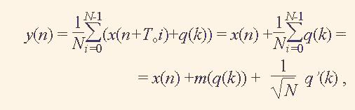 (3)
(3)
where m(q(k)) is the mean value of the noise q(k), q'(k) is the averaged noise signal without its mean value. We see obviously that the averaging can decrease the noise level in the signal up to √N times.
Due to this fact the averaging of the periodical signal is often used for the noise filtration. The serious conditions of this process are approaching to nil of the noise mean value and that the length of the accumulating array y(n), is equal to the х(n) signal period To .
Consider the periodical signal with the period То = N1 + N2 :
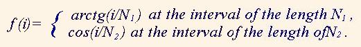
Then the unit which generates this signal is described as the following:
entity Gen is generic(n1:natural:=100;
n2:natural:=200);
port(CLK : in STD_LOGIC;
	RST : in STD_LOGIC;
	DATA_OUT : out REAL:=0.0;
	START : out BIT);
end Gen;
architecture MODEL of Gen is
signal ct2:natural;
begin
process(CLK,RST)	begin

if RST='1' then
		ct2<=0;
		START<='1';
	elsif CLK='1' and CLK'event then
		START<='0';
		if ct2=n1+n2-1 then
			ct2<=0;
		else
			ct2<=ct2+1;
		end if;
		if ct2<=n1 and ct2>0 then
	           DATA_OUT<= arctan(real(ct2)/real(n1));
		else
		   DATA_OUT<= cos(MATH_PI*real(ct2-n1)/real(n2));
		end if;
	end if;
end process;
end MODEL;
The network in the Fig.1 can be implemented as the test bench diagram in the Fig.2. This diagram is built using the Aldec ActiveHDL package.
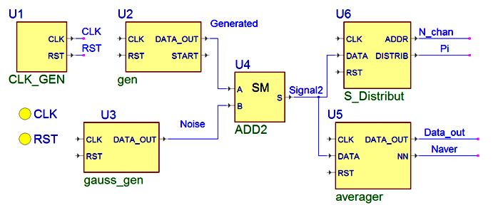
Fig. 3 illustrates signal, which is generated by the unit Gen, signal with added noise, and signal after 100 averaging cycles in the unit Averager. The analysis of the Fig.3 shows that after 100 averagings of the periodical signal the level of the added Gauss noise is really decreased in ca. 10 times.
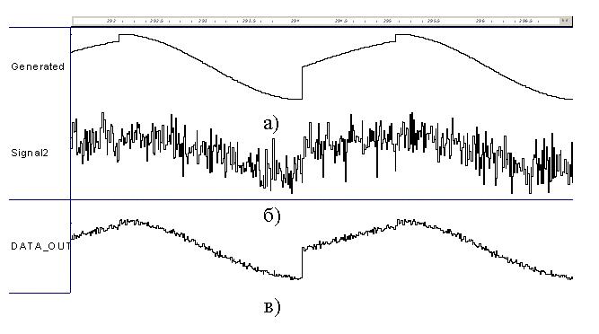
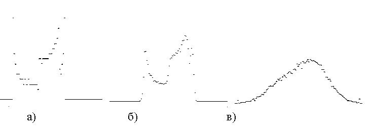
Fig.4 shows the diagrams of the output of the unit S_Distribut for the noise-free signal (Fig 3,a), signal with the added noise with the level 0.3, and level 3. The diagrams show that the signal has the positive mean value. The diagram Fig.4,a has the form, which characterizes the noise free signal, the diagram Fig.4,b shows that the noise is present in the signal. The diagram Fig.4,c shows that the noise level supersedes the signal level, and moreover, the noise has probably the Gauss distribution.
Conclusions. It is shown here http://kanyevsky.kpi.ua/ru/%D1%81%D1%82%D0%B0%D1%82%D1%8C%D0%B8/vhdl-%D0%BF%D1%80%D0%BE%D1%82%D0%B8%D0%B2-matlab/ that VHDL language has the wide opportunities to solve the different modeling problems especially at the field of DSP.