IIR filter analysis using VHDL.Allpass, multiple delay, and masking filters
A.Sergiyenko
National Technical University of Ukraine “КРІ”,
Email: aser@comsys.kpi.ua
z-transform and transfer function
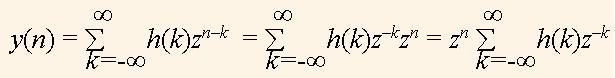
z-transform is widely used in DSP due to the fact, that the signal x(n) = zn is the eigenfunction of any linear system which is invariant to the signal shift. The eigenfunction means that when such a function is processed by the system then the output signal has the same form but is delayed, and its magnitude is different. We can show that zn is the eigenfunction of the system which is described by some impulse response h(k). Consider the signal zn is inputted to the system. Then due to the properties of the linear shift invariant system the output signal is
 (1)
(1)
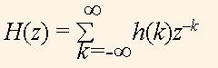
We see that the function zn passes through the system invariably. Due to the formula (1), the transfer function of the system is
 (2)
(2)
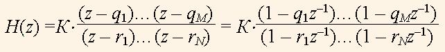
The function H(z) is the complex function with the magnitude |H(z)| and phase arg(H(z)). The function H(z) has two sets of special points. The first set contains the points q1,…,qM, for that |H(qі)| = 0. Therefore, these points are called zeros of the function H(z). The second set contains the points r1,…,rN, for that |H(rі)| = ∞, and therefore, they are called poles, of the function H(z).
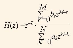
To find the poles and zeros of H(z), the sum (2) is transferred to the fraction with the positive powers of z. Such a fraction is the following
 (3)
(3)
The numerator and denominator of the fraction (3) are polynomials with the positive powers of z, and a0 = 1. The multiplier z-L represents the delay to L cycles, and can be taken off. The roots of these polynomials are equal to q1,…,qM and r1,…,rN,, and are called as zeros and poles, respectively. The function H(z) can be represented by the sets of zeros and poles as the following fractions
 (4)
(4)
where K is the transfer ratio or the amplification factor of the system.
Poles and zeros of the transfer function
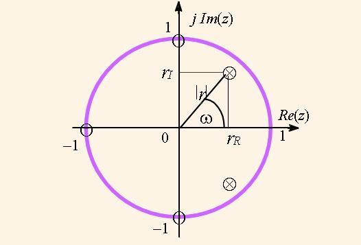
Poles and zeros are usually represented in the complex plane as circles and crosses respectively. Fig.1 illustrates an example of pole and zero allocation of some low pass filter. A root point is equal to a couple of real and imaginary numbers: r = rR + jrI . It is convenient to represent it in the polar coordinates by the magnitude |r|, and phase ω: r = |r|e-jω. When we consider the discrete signal computing the phase ω represents some frequency of the transfer function. The pole magnitude is not higher than a one for real filters, i.e. |r| < 1 . The number of poles with the nonzero imaginary parts is always even.
Magnitude-frequency response
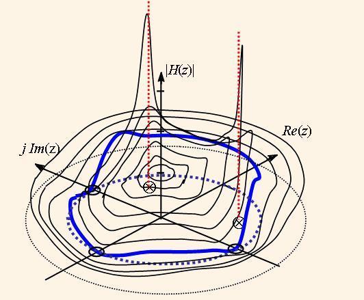
The magnitude of the transfer function |H(z)| can be represented in the three dimensional space as the endless elastic diaphragm, which is pulled up the complex plane at the mark one. The diaphragm points, which represent zeros, are pulled down to the complex plane, and points, which represent poles, are pulled up to infinity. If we draw the concentric circles in the diaphragm, then after its stretching we derive the figure like in the Fig.2. The bold line at the surface |H(z)| (Fig. 2) is mapped to the complex plane as a circle with the radius of one. This line is derived by
![]() (5)
(5)
When we input the sequence e-jω in the formula H(z), then we derive the discrete Fourier transform, and when we input it into formulas (2) or (3) we get the transfer function
|H(ω)| = |H(e-jω)|, (6)
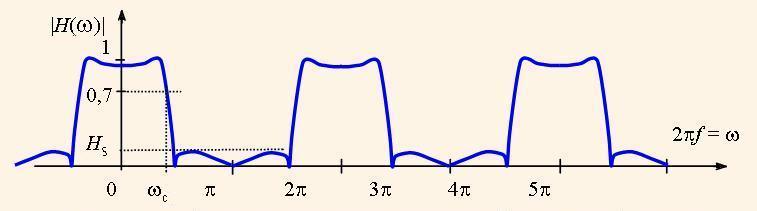
This transfer function means the transfer ratio dependence on the input signal frequency ω. The function |H(ω)| is called the magnitude frequency response (MFR) of the system. We can imagine that the bold curve in the Fig.2 is depicted in the cylinder, which is rotated on the axis o|H(z)|. When we untwist this curve and map it in the plane we derive the diagram, which is formed by the unlimited periodical curve with the period of 2π, like the curve in the Fig. 3.

The frequency axis of the MFR is normed by dividing to 2π for the usability, so as a one in this axis represents the sampling frequency.
Similarly the phase frequency responce (PFR) of the system is derived:
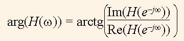 (7)
(7)
It is adopted for the digital filters, that they have the level of MFR higher than √0,5 ≈ 0,7 in the pass band. This means that in the pass band the power of the filtered signal is no less than a half of the nominal power. The respective frequency bound is called as the cutoff frequency (ωc in Fig. 3). The maximum level of the filtered signal in the stop band is called the suppression level of the filter (Hs in Fig.3).
The DSP systems are usually the chains of sequentially connected units.
Therefore, it is useful to represent MFR with the logarithmical scale, i.e.
H(ω) = 20*lg|H(e-jωn)|
Then the resulting MFR of the system is equal to the sum of MFRs of its parts. The level of such MFR is measured in decibels. For example, the level H(ω) = 1 represents 0 db, level 0,7 means -3 db., level 0,5 means -6 db, and so on.
Allpass filters
Further for the instance we will investigate the transfer function of the form
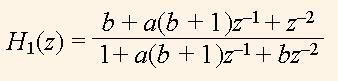 (8)
(8)
and other functions based on it. Function H1(z) represents the allpass filter. The poles and zeros of the function H1(z) are illustrated by Fig. 4. The poles and zeros of the function (8) have the equal angles ω. If length of the pole vector is equal to r, then the length of the zero vector is equal to 1/r. As a result, the zeros fully compensate the poles, and MFR is equal to 1 in the whole frequency band. For this property such a filter is called as an allpass one.
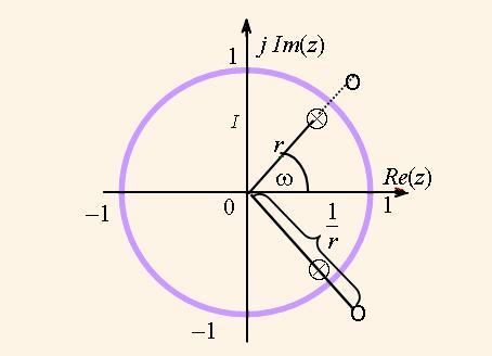
The factors a and b determine the zero and pole coordinates due to the formulas
a = – cos(ω); b = r2. (9)
The allpass filter has not effect on the signal magnitude, but it distorts cardinally its phase. Moreover, when the factor b approaches to a one, then the phase distortion at the frequency ω is sharper. If we connect two allpass filters with the characteristics H1(z), H2(z) in parallel, i.e.
H3(z) =(H1(z) + H2(z))/2, (10)
then the poles and zeros in the resulting characteristic H3(z) stop to compensate each other. Both cannels H1(z), H2(z) pass the input signal without its magnitude exchange. But on the frequency, where the phase difference is equal to π, 3π,…,, the output signals compensate each other and the resulting signal is zero. On the contrary, on the frequency, where the phase difference is equal to 0,2π, 4π,…, the resulting signal is doubled after addition. This causes the division to the factor 2 in the formula (10). As a result, the pass band and stop band are present in MFR |H(ω)|.
Multiple delay filters and masking filters
One can increase all the delays in k times in the linear DSP system. Then instead of the transfer function H(z) the function with multiple delays H(zk) is considered. For this feature such a filter is named as a multiple delay filter. The effect of delay multiplication consists in scaling MFR, and PFR diagrams in k times along the axis of frequencies.
Let the coefficient k is equal to 2, then in the diagram in the Fig. 3 the marks π, 2π and so on are exchanged to marks π/2, π etc. As a result, the number of both pass bands and stop bands is doubled.
Consider H3(z) is a low pass filter, and we construct the multiple delay filter H4(z) = H3(zk). Then its MFR |H4(ω)| has k pass bands. In this situation we can select a single working pass band using, so called, masking filter with the transfer function HM(z). Such a filter is connected to the multiple delay filter in sequence, i.e. the resulting transfer function is
H(z) = H4(z)*HM(z) (11)
MFR of the masking filter has the stop bands in that frequencies where the pass bands in MFR |H4(ω)| are present, which we want to suppress.
Some useful VHDL functions
In this article we consider the computation of the transfer functions using VHDL. For this purpose we have to use the mathematical packages IEEE.MATH_REAL, and IEEE.MATH_COMPLEX. In the last package the constants, types, and functions are defined, which operate with the complex data.
Below we consider a set of developed functions, which are useful to calculate the transfer function. The calculation of the sequence zn is implemented using the following functions, which overload each other.
--complex vector Z with magnitude MAG, and phase  j*fi
 function Z(mag,fi:real) return COMPLEX_POLAR is
    begin
 return mag*exp(COMPLEX_TO_POLAR(MATH_CBASE_J)*(fi));
 end Z;
--complex number Z with magnitude 1, and phase  j*fi
 function Z(fi:real)  return COMPLEX_POLAR is
    begin
 return exp(COMPLEX_TO_POLAR(MATH_CBASE_J)*(fi));
 end Z;
The following function calculates H1(z) due to the formula (8), but for positive degrees of z , i.e. considering the equation(3). It is useful for the scanning of the space |H1(z)| when we search for zeros and poles. By this process we sequentially set different values of the magnitude mag, аnd phase fi of the complex vector z. It is used for computations of MFR and PFR as well.
calculating (bZ^2+а(b+1)Z+1)/(Z^2+c(b+1)Z+b)
 function Allpass2(b,a: real; --coefficients
 	mag, fi: real)  -- magnitude, angle for z
     return COMPLEX_POLAR is
	variable tn,td:	COMPLEX_POLAR;
     begin
	td:=COMPLEX_TO_POLAR(COMPLEX'(b,0.0))
	+a*(b+1.0)*Z(mag,fi) + Z(mag**2,2.0*fi);
	tn:=COMPLEX_TO_POLAR(COMPLEX'(1.0,0.0))
	+a*(b+1.0)*Z(mag,fi) + b*Z(mag**2,2.0*fi);
	return tn/td ;
 end Allpass2;
The following function calculates the formula H1(z2) (8) for the negative degrees of z with a single magnitude, i.e. it calculates the function H1(ω), for ω = fi . Therefore, it is used only for computing MFR, and PFR.
 function Allpass2x2(b,c:real; fi:real)
 return COMPLEX_POLAR is
	variable tn,td: COMPLEX_POLAR;
 begin
    tn:=COMPLEX_TO_POLAR(COMPLEX'(b,0.0))
       +c*(b+1.0)*Z(-2.0*fi) + Z(-4.0*fi); --numerator
    td:=COMPLEX_TO_POLAR(COMPLEX'(1.0,0.0))
       +c*(b+1.0)*Z(-2.0*fi) + b*Z(-4.0*fi); --denominator
	return tn/td ;
 end Allpass2x2;
To scan the three dimensional space |H1(z)| the following part of the VHDL program is used.
 signal clk:bit;
 signal m,ph:real:=0.0;
 signal a,b,logm,phase,mag:real:=0.0;
 begin
    clk<=not clk after 5ns; --clock generator
 process(CLK)
   variable p,phas:real:=0.0;
   variable Hz: COMPLEX_POLAR;
   begin
       	a<=-0.5;  b<=0.64;    -- parameters of H(z)
    if clk='1' and clk'event then
	phas:= phas+0.001; -- phase counter (frequency)
	p:=phas*MATH_PI*2.0; 	-- normed phase
	m<= trunc(phas)*0.1+0.1; -- magnitude of Z
	ph<=phas;         	-- phase signal
    end if;
        Hz:=Allpass2(b,a,m,p);  --resulting H(z)
        mag<=abs(Hz);		-- magnitude of H(z)
        phase<=Hz.ARG;		-- phase of H(z)
        logm<=20.0*log10(abs(Hz)); -- H(z) in decibels
  end process;
Investigation of the allpass filters using VHDL
Let us investigate the function H1(z) using the VHDL program, which outputs the diagrams |H1(z)| for different values |z| to estimate the coordinates of poles and zeros of the function (7). Consider a = -0.5, b = 0.64. Then the transfer function is
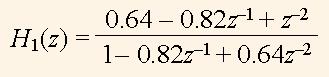 (12)
(12)
After running the described above VHDL program in the system Aldec ActiveHDL the diagram |H1(z)| (Fig. 5) was outputted. In this diagram the curves |H1(m,ph)| are placed in a set of intervals, marked as m, where m = 0.1, 0.2,…, is magnitude, ph is phase (frequency) of the vector z. The vector z makes a single turnover when ph is exchanged from i to i+1, where i is the number of the interval. The first diagram |H1(m,ph)| on the Fig. 5 is built for m = 0.1,...0.9, and the second one is for m = 1.0,...1.9. We can see that each interval represents an exclusive curve like ones in the Fig. 2. In the Fig.5 the diagram arg(H1(z)) for m = 0.6,...1.1 is shown as well.
The analysis of the diagrams in the Fig. 5 shows the following. We see, that the magnitude of H1(z) at m = 1 is really equal to a one. The poles of the function H1(z) have the measured phases ± 2π*ph = ± 2π*0.1645 = ± 1.0336, and they have the polar coordinates r1 = 0.8 ∠1.0336 and r2 = 0.8 ∠-1.0336. The zeros of the function H1(z) have the same phase and are equal to q1 = 1.3 ∠1.0336, q2 = 1.3∠-1.0336. One can see that -cos(1.0336) = -0.512 ≈ a, 1/0.8 = = 1.25 ≈ 1.3, and 0.82 = 0.64 = b, i.e. the formulas (9) are true.
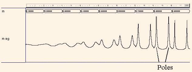
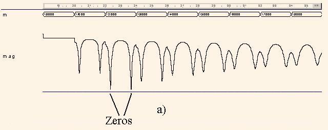
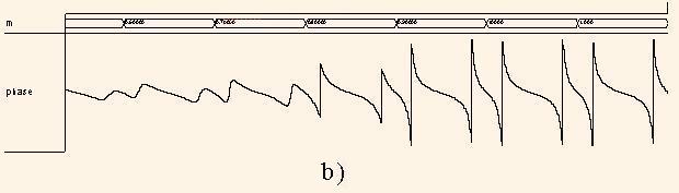
Fig. 5. Involute of the function |H1(z)| (a) and of the function arg(H1(z)) (b)
The analysis of the diagram arg(H1(z)) shows that for the angles ph = 0 the phase is equal to 0, and for the gradual increase of ph the resulting phase is monotonously decreased. But when ph and norm of z approach to poles the phase sharply approaches to ±π.
Let us analyze the function H3(z) by H2(z) = z-1 . Here H2(z) = z-1 is the transfer function of another allpass filter, because |H3(z)| = 1 for all z.
To compute the function | H3(ω)| in the previous VHDL program one variable assignment operator is substituted to the following operator, which represents the formula (10) .
Hz:=(Allpass2(b,a,1.0,p)+Z(-1.0*p))/2.0 (13)
Some correction of the factor b is made, i.e. = 0.625. The resulting function is
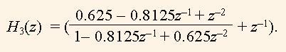 (14)
(14)
One can show that the multiplication to the multiplier 0.625 can be implemented as a single addition of the multiplicand, which is shifted right to one and three bits respectively. Similarly the multiplication to a factor 0.8125 can be made. This feature simplifies substantially the hardware of the filter, which is represented by the formula (14).
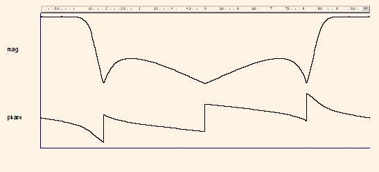
After the running of this program the diagrams |H3(ω)| and arg(H3(ω)) are derived for the frequencies ω=(0, 2π) or for the normed frequencies ph = (0, 1), which areshown in the Fig.6. We can see that after addition of the functions H1(z) and H2(z) the function of the low pass filter is obtained. Due to the diagram this filter has the cut-off frequency fc = 0,156 ≈ arg(r1) =1/(2π) 1,0336 = 0,164, and the suppress level of 8.5 db.
Now we can investigate the function H4(z).
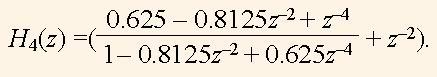 (15)
(15)
The diagram |H4(ω)| (Fig.7,а) is built by the substitution of an operator to the following one as well as in the previous example.
Hz:=(Allpass2x2(b,a,p)+Z(-2.0*p))/2.0;
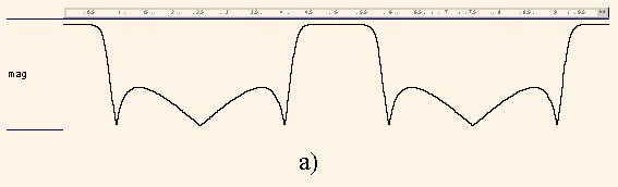
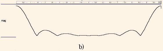
Fig. 7. Diagrams of the magnitude frequency responses |H4(ω)| (a), |HM(ω)| (b), |H(ω)| in the linear and logarithmical scales
We can see that the diagram in Fig.7,a represents the twofold repeated diagram in Fig 6, which is typical to the filters with multiple delays.
Тhe function of the masking filter
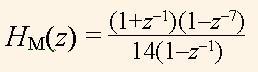 (16)
(16)
we can prove by the diagram |HM(ω)| (Fig.7,b), which is computed using the following operator.
 Hz:=(COMPLEX_TO_POLAR(COMPLEX'(1.0,0.0))+Z(-p))
    *(COMPLEX_TO_POLAR(COMPLEX'(1.0,0.0))-Z(-7.0*p))/
     (COMPLEX_TO_POLAR(COMPLEX'(1.0,0.0))-Z(-p))/14.0;
Finally we can investigate the function (11), which is the composition of functions H4(z) and HM(z):
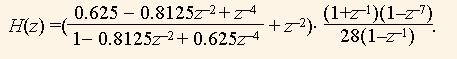 (17)
(17)
The diagram of resulting MFR |H(ω)| (Fig.7,c) is generated using the following operator.
 Hz:=(Allpass2x2(b,a,p)+Z(-2.0*p))
      *COMPLEX_TO_POLAR(COMPLEX'(1.0,0.0))+Z(-p)
      *COMPLEX_TO_POLAR(COMPLEX'(1.0,0.0))-Z(-7.0*p))/
       (COMPLEX_TO_POLAR(COMPLEX'(1.0,0.0))-Z(-p))/28.0;
As we can see in Fig.7, the function HМ(z) masks the function H4(z). As a result, we derive the transfer function H(z) of the low pass filter which cutoff frequency is equal to fc = 0,06 and suppression level is higher than 23 db.
Concluding the article we can see that the simple transfer function (12), which can be implemented only with additions, has rather high filtering properties. The FIR filter with the analogous characteristics has at least the order 60. The properties of this function were investigated by using only VHDL, not to consider Matlab or other popular DSP modeling tools.
Further data about allpass filters, masking and multiple delay filter one can find in the references below.
References
1. Chung J. G., Parhi K. K. Pipelined wave digital filter design for narrow-band sharp-transition digital filters // Proc. IEEE Workshop VLSI Signal Processing, La Jolla, CA. –1994. –Р. 501-510.
2. Regalia P., Mitra S.K., Vaidyanathan P.P. The Digital All-Pass Filter: A Versatile Signal Processing Building Block // Proc. IEEE. –1988. –V.76. –№1. – p.19-37.